i4Q Digital Twin

General Description

i4QDT (Digital Twin Simulation Services) allows industrial companies to achieve a connected 3D production simulation, with a digital twin for manufacturing enabling virtual validation/visualisation and productivity optimisation using data from different factory levels (small cell to entire factory).

i4QDT is able to provide a virtual representation and contextualization of all the assets present in a manufacturing line. The virtual representations of the different physical devices are accessible through APIs, creating a framework of consistent interoperability that allows the building of the digital twins in a more focused digital twin domain, and reducing the complexity of IoT deployments. Additionally, when virtual sensors are to be obtained, physics-based models are developed. An industrial model exchange standard is used for facilitating the integration of models with monitoring algorithms, protecting the model intellectual property, and making the framework independent from the modelling source.

Features

This i4QDT Solution offers following features:

• Provides the capability of building models and stablishing the relationships between the inputs of the model and the collected data (contextualization).

• Provides the capability of loading, storing and updating individual models representing the different sections and machines of a plant.

• Provides the capability of running simulations of both data-driven models (machine learning python models) and physics-based models (FMU compiled models).

• Provides the capability of storing and visualizing the results from the simulations.

Comercial information

Authors

Partner	Role	Website	Logo
IKERLAN	Leader	www.ikerlan.es/en/
CERTH	Participant	https://www.certh.gr/root.en.aspx

Technical Specifications

i4QDT is a docker container allowing to launch simulations of a manufacturing asset/plant based on production/machine data and their digital twin (DT) and obtain results that are visualized in a 3D environment and other data visualization formats (graphs/tables). Each DT allows calls to perform simulations that can be managed through REST APIs. It gives inputs to other solutions such as i4Q Prescriptive Analysis Tool and i4Q Line Reconfiguration Toolkit. The i4QDT is comprised of three main software packages: physics-based back end, data-driven back-end and user interface back-end. The physics-based workflow makes use of Functional Mock-up Units (FMU) that have been compiled from different modelling languages like Modelica, which are component-oriented and based on a set of equations defining the physics behaviour of the system. The data-driven approach designed and developed within the implementation phase of i4QDT correspond to machine learning methods, comprising data-driven machine learning techniques, which are highly promising since a model learns critical insights directly and automatically from the given datasets.

Technical Development

This i4Q Solution has the following development requirements:

• Language: Python

• Libraries: Numpy, Pandas, Matplotlib, Networkx, FMPy, Pyyaml, Flask

• Orchestration: Docker

• Technology area: FMI, Modelica -

• Programming interface: RestAPI - User interface front-end: React, PrimeReact, Redux

License

• Dual License AGPLv3 or PRIVATE

Pricing

• Quotation under request

Associated i4Q Solutions

Optional

• i4Q Data Repository

• i4Q Message Broker

• i4Q Data Integration and Transformation Services

• i4Q Prescriptive Analysis Tools

• i4Q Line Reconfiguration Toolkit

System Requirements

• Docker Desktop for Windows

• Docker Desktop for Mac

Installation Guidelines

Resource	Location
Last release (v.1.0.0)	Gitlab Project
Node.js	Link

i4QDT docker installation

• Dowload the zip file from this link: [Download]

• Create a new folder in your local computer and extract the content of the zip file so the structure is as follows:

New folder
|
|---- Front-end
|     |-- Dockerfile
|
|---- Backend
|     |-- Dockerfile
|
|---- docker-compose.yaml

• Open a new terminal in the folder where the docker-compose file is located and run the following command:

docker-compose up --build

• The application will be running as soon as the process finishes. The url where the user interface is running will be shown in the terminal, which by default is http://localhost:8082

• In order to stop the application the terminal needs to be closed.

i4QDT front-end installation (optional)

Install project dependencies, open a terminal in frontend folder:

cd \subsystems\frontend
npm install

User Manual

The following user manual is divided into three sections: the API specification, the description of the front-end and the fmiSim User Manual (this last one only in case someone wants to use it separately from the i4QDT solution).

API specification

To start the server application on a local computer, a tab in the default browser will be opened. Then the following line should be entered in shell.

python scr/app.py

This action starts a server running in port 5000 and allows to use the following API methods. Those methods are accesible through the application front-end or sending the proper request using any other tool like Postman, or directly with Python code:

Resource	POST	GET	PUT	DELETE
/FMUListResource	Adds the fmus selected to the Master	Sends a list of the available fmu models in the internal folder of the API
/VariableResource		Extracts the internal parameters and variables of each of the fmus of the master
/uploadFMU	Uploads and saves into an internat folder any fmu selected by the user		Reloads the Master
/Simulation	Receives simulation parameters and executes the simulation of the fmus in the Master		Adds connections between the fmus	Supported
/ExternalInput	Loads a csv file with input values for a fmu			Supported

In the following sections the API functions are described both for physics-based workflow and for data-driven workflow:

APIs for physics-based models parametrization and simulation

• FMUListResource (URL: “/load_fmu”):

  • GET: Sends a list of the available fmu models in the internal folder of the API.

    • Response type: {“data”: [ { “name”: “addSignals.fmu” }, { “name”: “Bouncing_ball_simple_21b.fmu” } ] }

  • POST: Adds the fmus selected to the Master.

    • Request type : {‘selected_models’: [{‘name’: ‘addSignals.fmu’}, {‘name’: ‘Bouncing_ball_simple_21b.fmu’}]}.

    • Response type: {‘message’:‘post fmulist resource’}

• VariableResource (URL: “/get_variables”):

  • GET: This method extracts the internal parameters and variables of each of the fmus of the master

    • Response: {‘variables’: {Internal variables of the fmu}}}

• uploadFMU (URL: “/upload_fmu”):

  • POST: This method uploads and saves into an internat folder any fmu selected by the user.

    • Request type: To make a request of uploading a fmu trought Postman follow this steps:

      1. Create a new post request with the url https://localhost:5000/upload_fmu

      2. Add a file as form data: In the Body tab, select the form-data option.Then hover your mouse over the row so you can see a dropdown appear that says Text. Click this dropdown and set it to File, and write “fmu[]” in that cell.

      3. A “Selected Files” option shoud have been appeared in the VALUE tab. Click it and select one or more files.

      4. Send the request.

    • Response: {‘message’: ‘Uploaded succesfully’}

  • PUT: Reloads the Master. This action will reset the master, removing any fmus it previously had.

    • Request type: {‘reset_master’: true}.

    • Response: {‘message’: ‘Master Reloaded’}

• Simulation (URL: “/simulation”):

  • POST: This method receives simulation parameters and executes the simulation of the fmus in the Master.

    • Request type: The request must must contain the summation of 3 components:

      1. Simulation start values: list of dictionaries with the start value of the desired input variable and the model to which it belongs.

      2. Output variables: list of dictionaries with the desired output variable and the model to which it belongs.

      3. Simulation parameters: a dictionary with the start time, the stop time and the step size.

      An example is shown:

      {‘simulation_start_values’: [{‘model_identifier’: ‘gainInput1’, ‘code’: 0, ‘items’: [{‘variable’: ‘inputGain1’, ‘start’: ‘0.0’}, {‘variable’: ‘gain1.k’, ‘start’: ‘5.0’}]}, {‘model_identifier’: ‘pulseForce’, ‘code’: 1, ‘items’: [{‘variable’: ‘pulseForce.nperiod’, ‘start’: ‘1’}]}], ‘simulation_selected_output_variables’: [{‘model_identifier’: ‘gainInput1’, ‘variable’: ‘inputGain1’}, {‘model_identifier’: ‘pulseForce’, ‘variable’: ‘forceOutput’}], ‘simulation_parameters’: {‘start_time’: 0, ‘stop_time’: 10, ‘step_size’: 0.2}}.

    • Response: {‘ModelOutputs’: modelOutputs}

  • PUT: Add connections between the fmus.

    • Request type: list of dictionaries with the output variable and it’s model and the input variable and it’s model, separated by “/”. An example is shown: {‘models_connections’: [{‘name’: ‘pulseForce.forceOutput / gainInput1.inputGain1’}]}.

    • Response: {‘ModelOutputs’: ‘Connections added’}

• ExternalInput (URL: “/upload_Input_Signal”):

  • POST: Loads a csv file with input values for a fmu. This method should be used if the input for a model varies through time.

    • Request type: The steps to make a request of loading a csv file are the same as in uploadFMU request, being the KEY “inputSignal”. AN example of how it should be the structure is presented:

      time	addSignals.inputSignal1	addSignals.inputSignal2
      0	0	0
      0,1	0	1
      0,2	1	0
      0,3	1	1
      0,4	0	0

      Considerations:

      • The first column must always be “time”.

      • time-steps and values must always be separated by “,”.

      • The column names must be named with the name of the model followed by the name of the variable, both separated by a dot.

      • Each cell must contain the variable value for the given time-step.

      • The variables in the csv must belong to models previously uploaded to the master.

    • Response: {‘message’: ‘Uploaded succesfully’} #### APIs for data-driven workflow WORK IN PROGRESS

Front-end User Manual

To start application on localhost, a tab in the default browser will be opened:

npm start

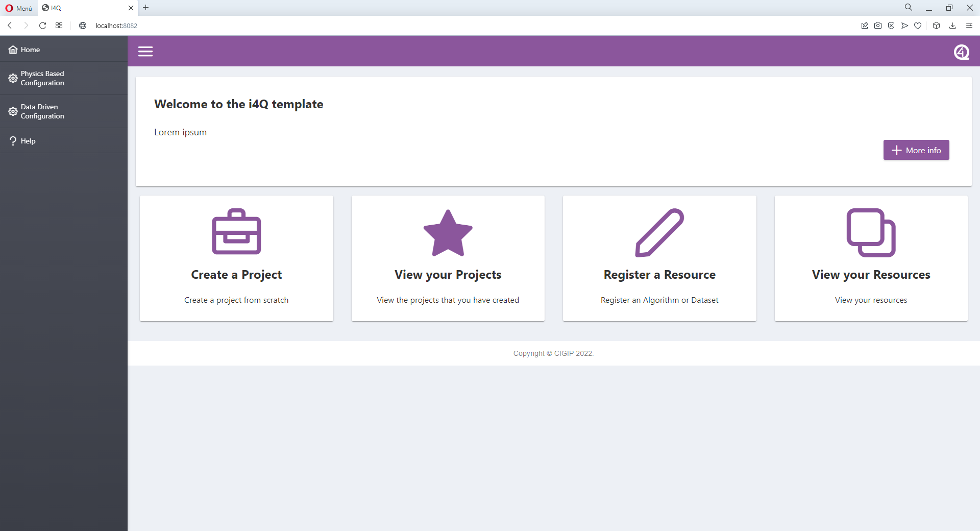
Application will open in its home screen, there are 2 main screens that can be access through the application left side menu: - Home Screen - where an introduction of i4QDT is displayed.

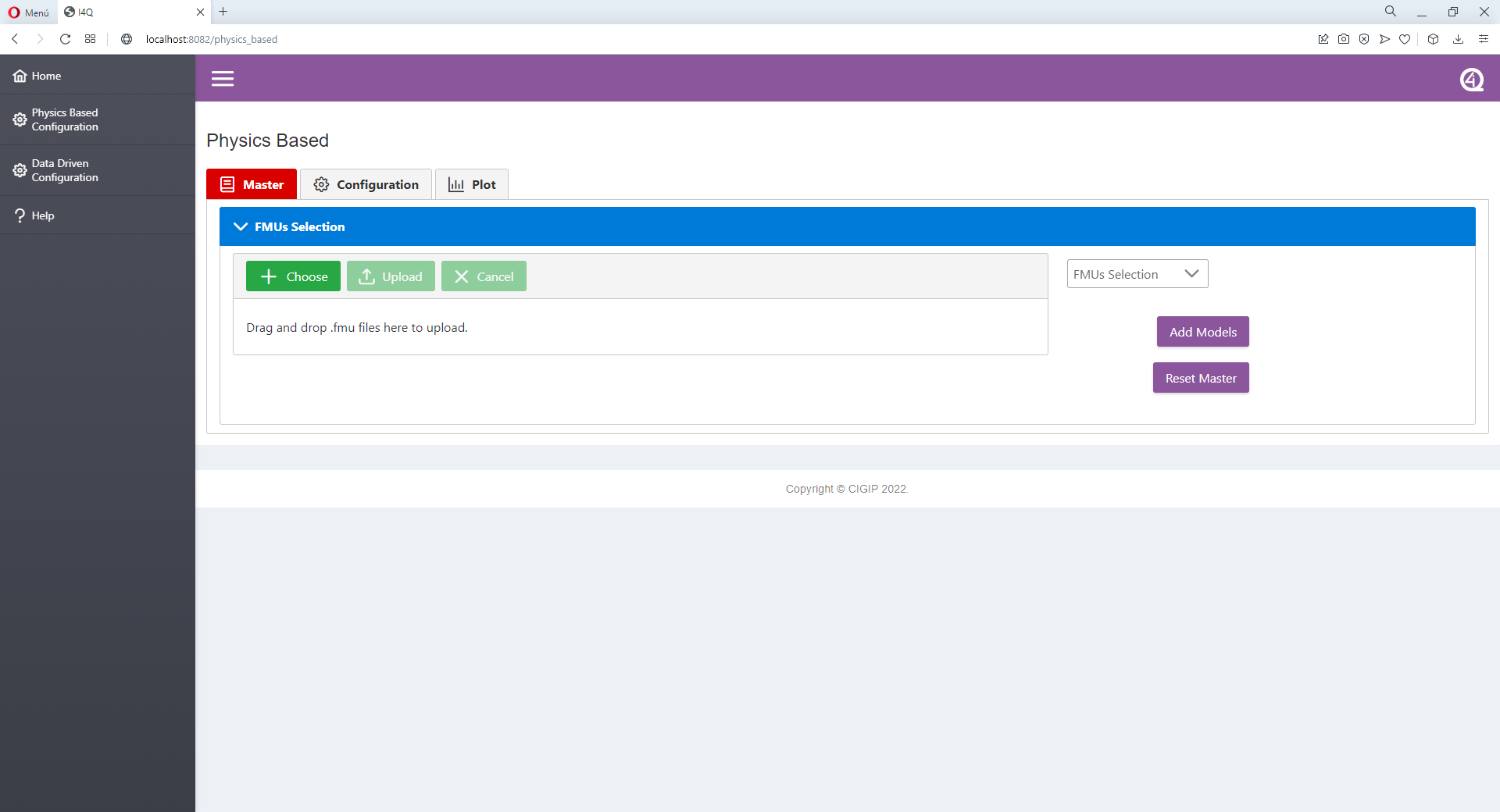
-Physics-Based Screen - where physics-based models can be parametrized and simulated.

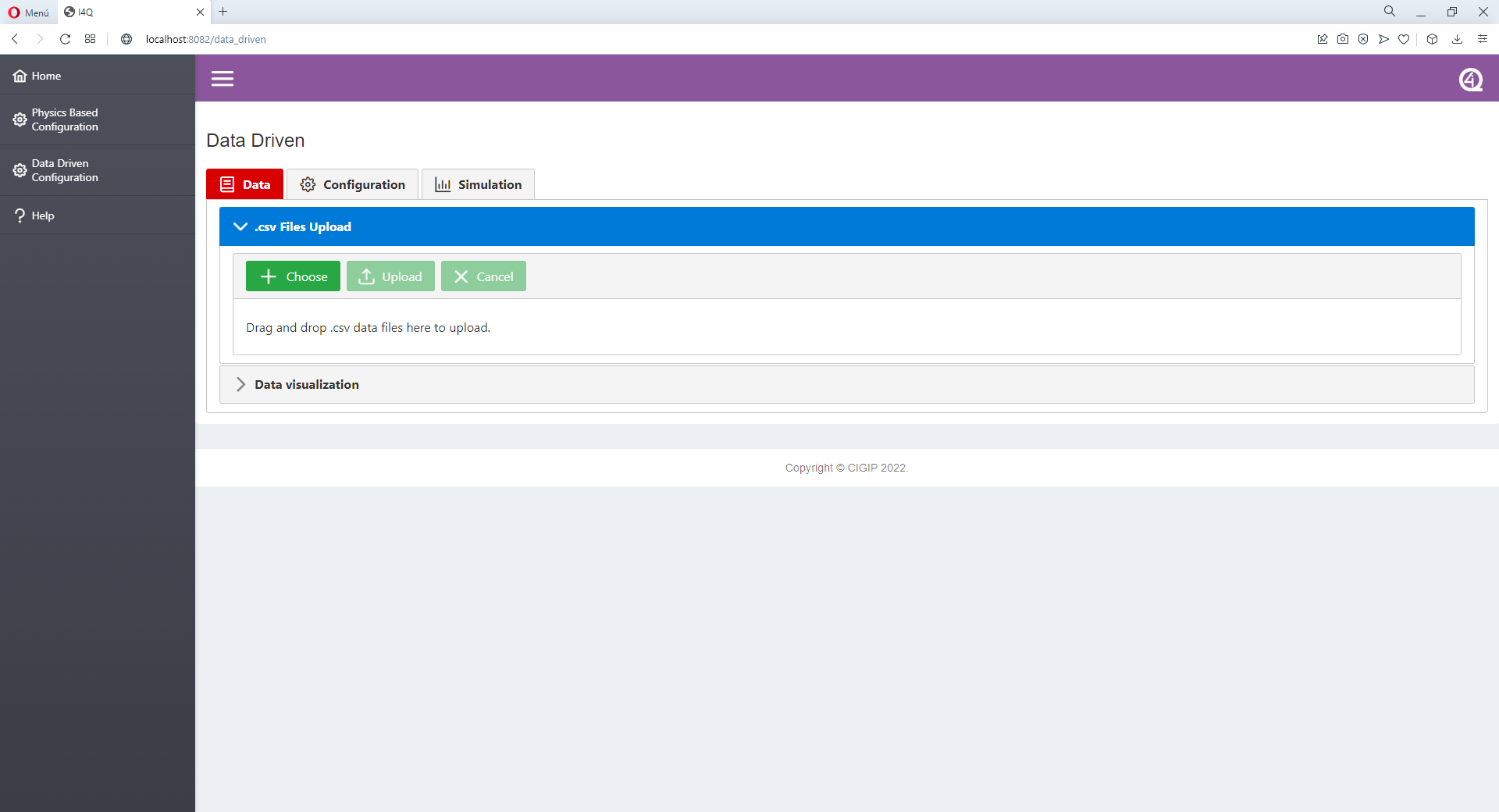
• Data-Driven Screen - where data-driven models can be parametrized and simulated.

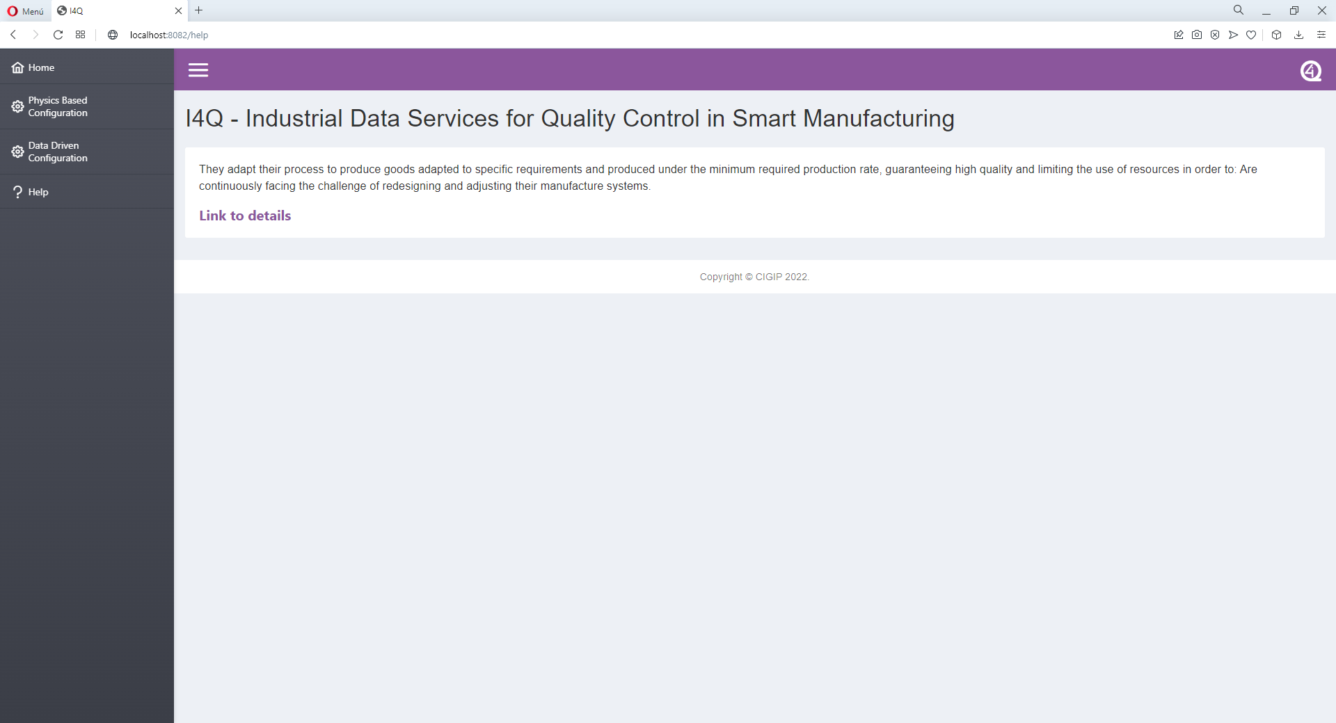
• Help Screen - where guidelines for the user are displayed.

Two main tasks can be perform depending on user needs:

For physics-based models parametrization and simulation * Uploading FMU files (Master TAB).

1. Click “Choose” button or drag and drop FMU files from your computer.

2. The select FMUs and its size will be displayed as a list.

3. To have this FMUs available on the FMUs dropdown list click “Upload” button, otherwise click “Cancel” button to clean the file uploader.

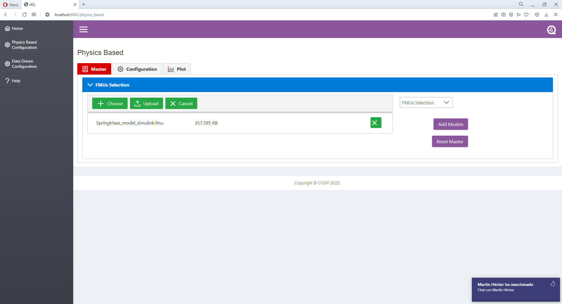
• Adding Models to the Master (Master TAB).

1. Select the desired FMUs from the FMUs dropdown list.

2. Click “Add Models” to add the selected FMUs to the Master.

3. To reset current Master configuration click “Reset Master”. It will delete all current configurations.

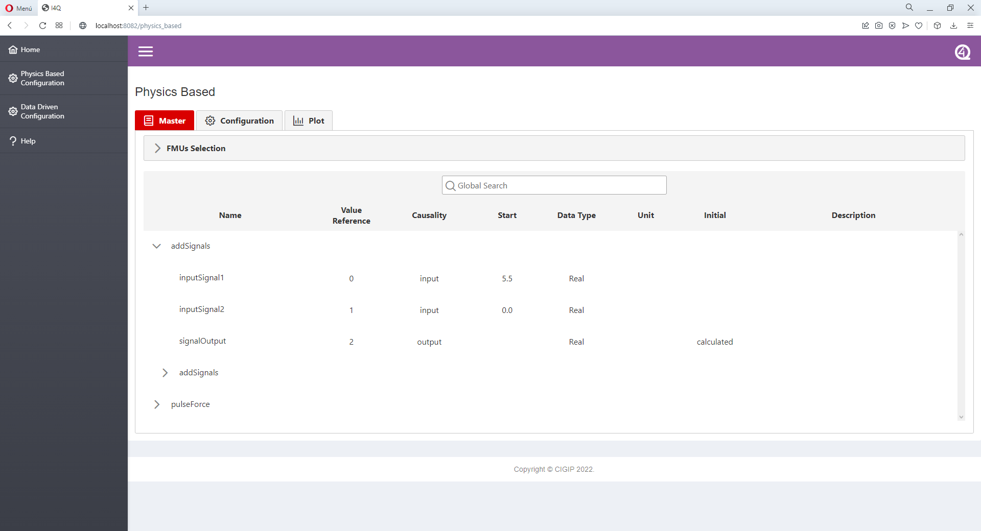
• Modifying Models start values (Master TAB).

1. Once Models have been added to the Master they will be displayed in a tree table format.

2. Input variables start values can be modified. If input variable start value is clicked, and input field will appear and user interaction is allowed.

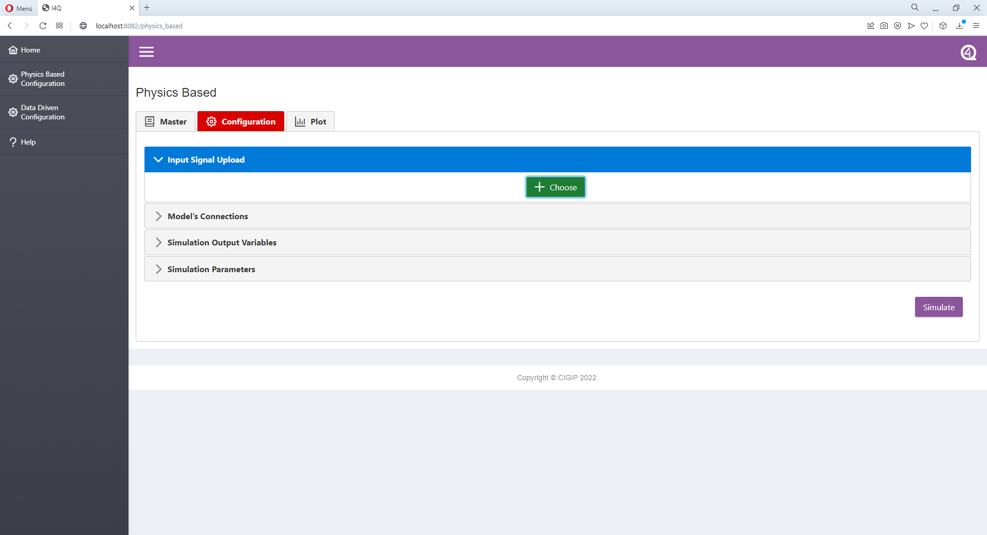
• Uploading an input signal (Configuration Tab).

1. Similar to the file uploader for FMUs, users can select a .csv file with an input signal to be used in the simulation.

2. Once selected and uploaded, the signal data is displayed in table format.

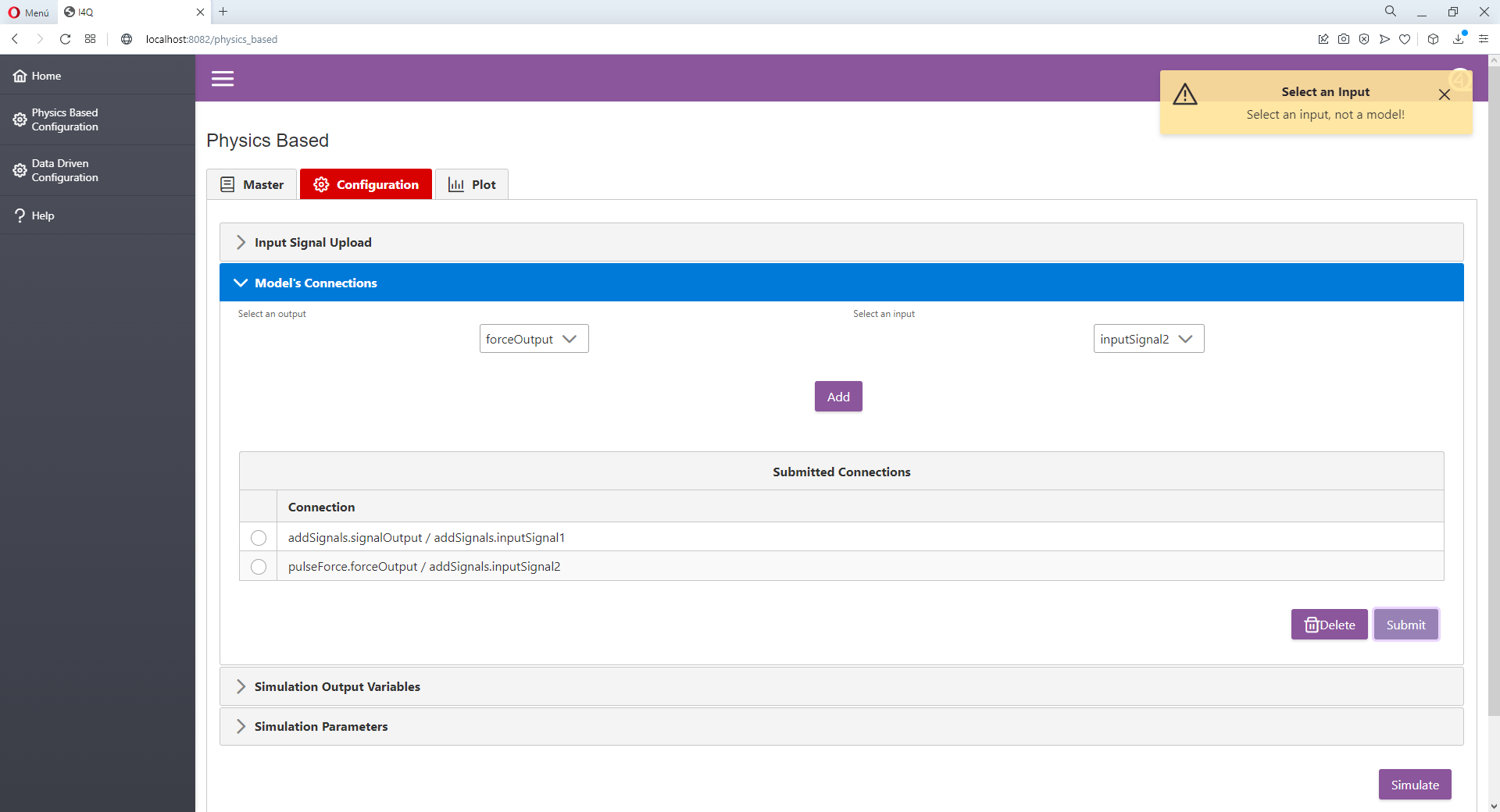
• Configurating model’s interconnections (Configuration Tab).

1. Two dropdown lists are displayed, one for outputs, the other for inputs, where user can define the interconnections. Once define the connection from the selected output to the selected input and click “Add” button, the define connections will be displayed in a table format.

2. In order to delete a connection select the desired connection and click “Delete” button.

3. Once all connections are defined click “Submit” button to send this information to the Master.

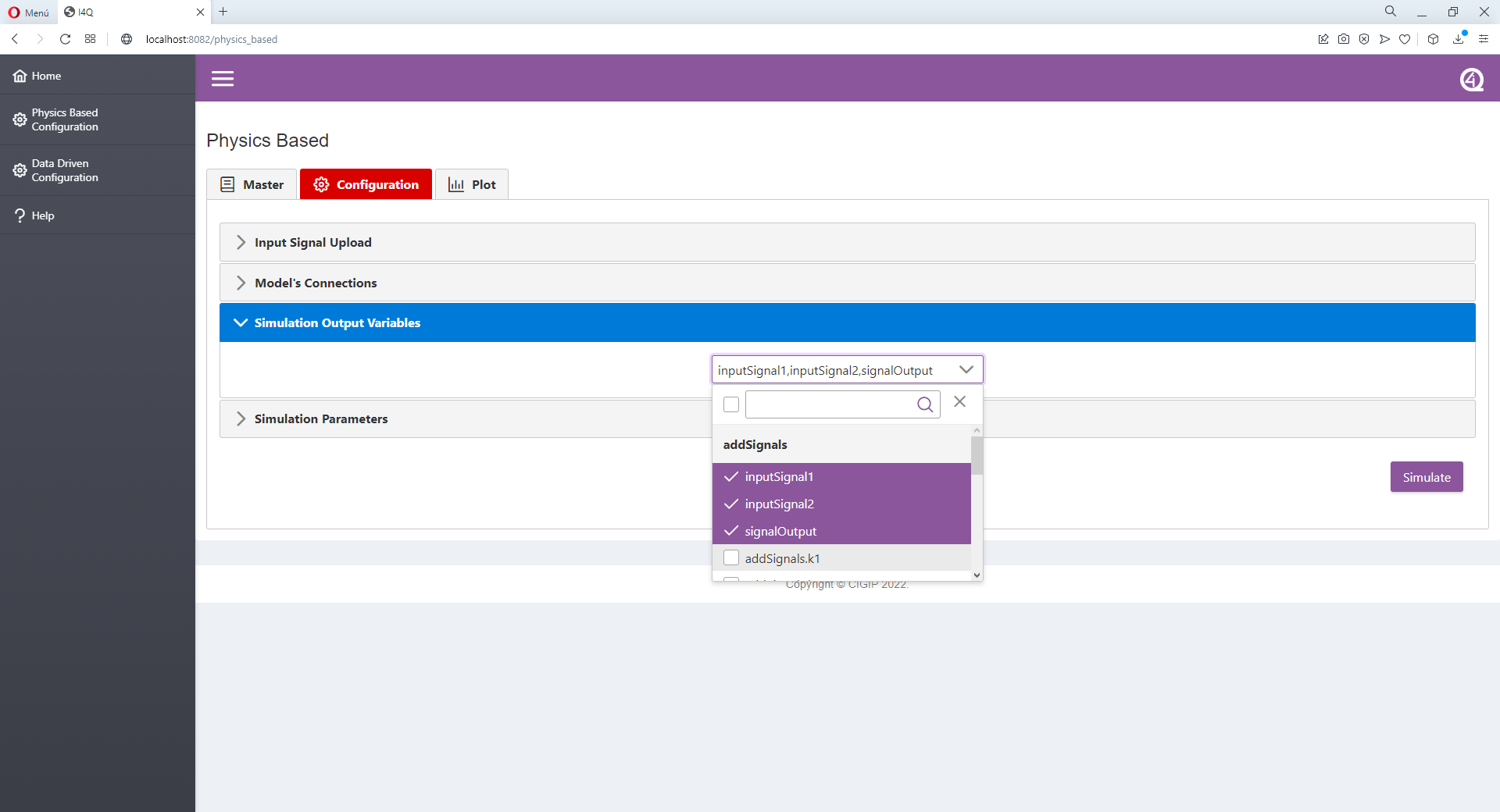
• Selecting the simulation output variables (Configuration Tab).

1. Variables can be selected from a dropdown list contaning all models variables added to the master.

• Simulation Parametrization (Configuration Tab).

1. Where the user can parametrize: the simulation start time, the simulation stop time and the simulation step size.

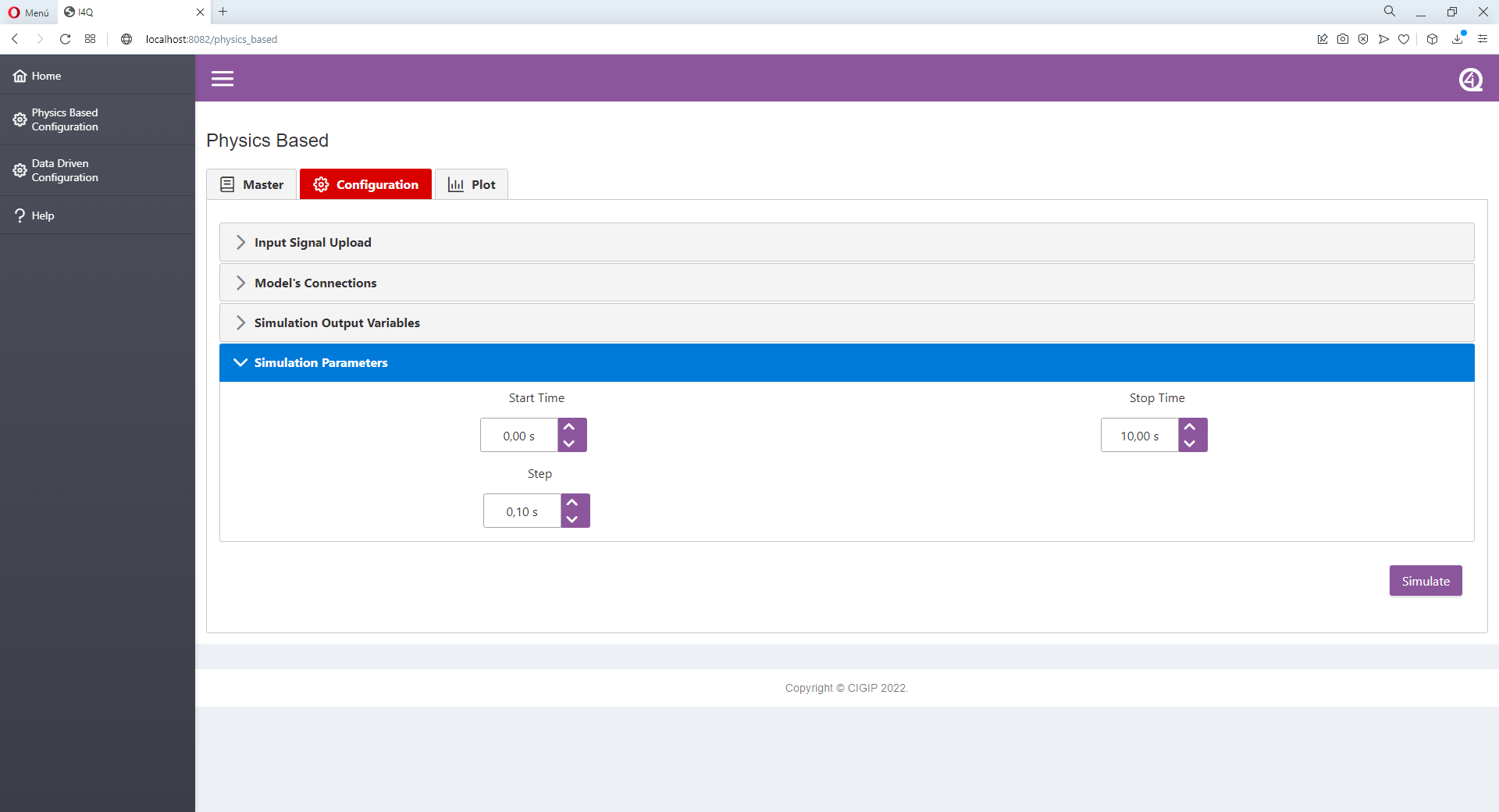
• Click “Simulate” button to start the simulation (Configuration Tab).

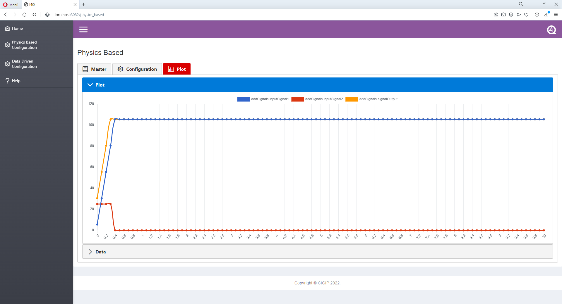
• Simulation results (Plot Tab).

1. A scatter/line plot is displayed with the variables selected before.

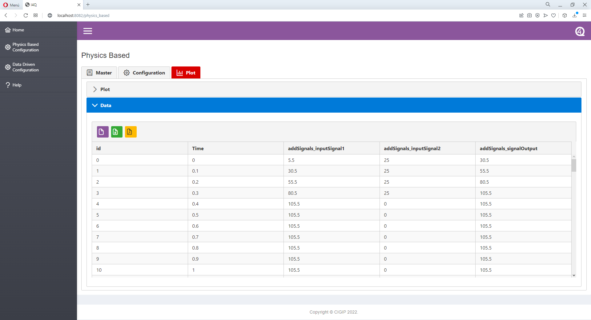
2. This same data is also displayed in table format.

3. This data can be downloaded as: .csv, .xlsx and .pdf.

For data-driven models parametrization and simulation

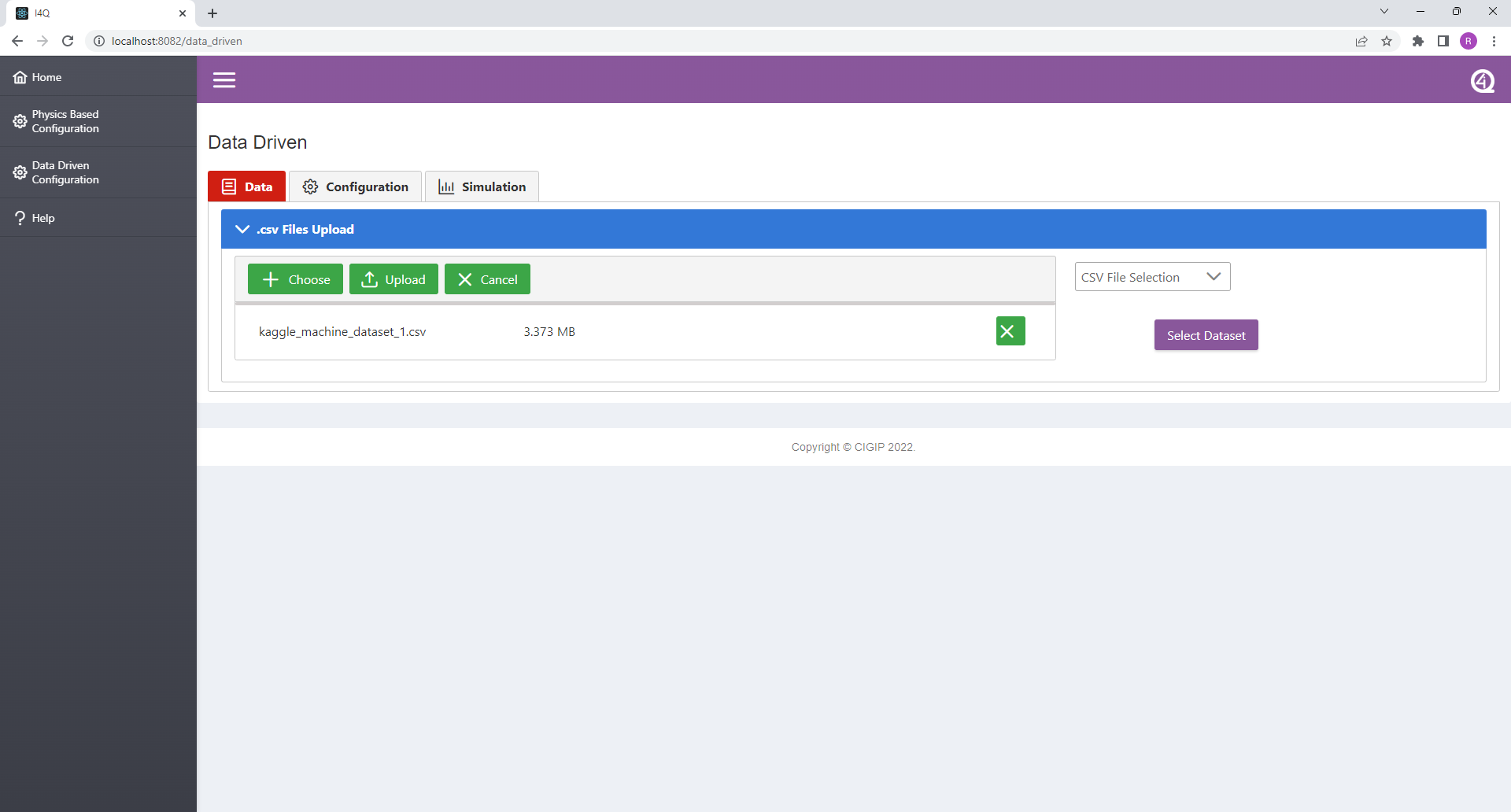
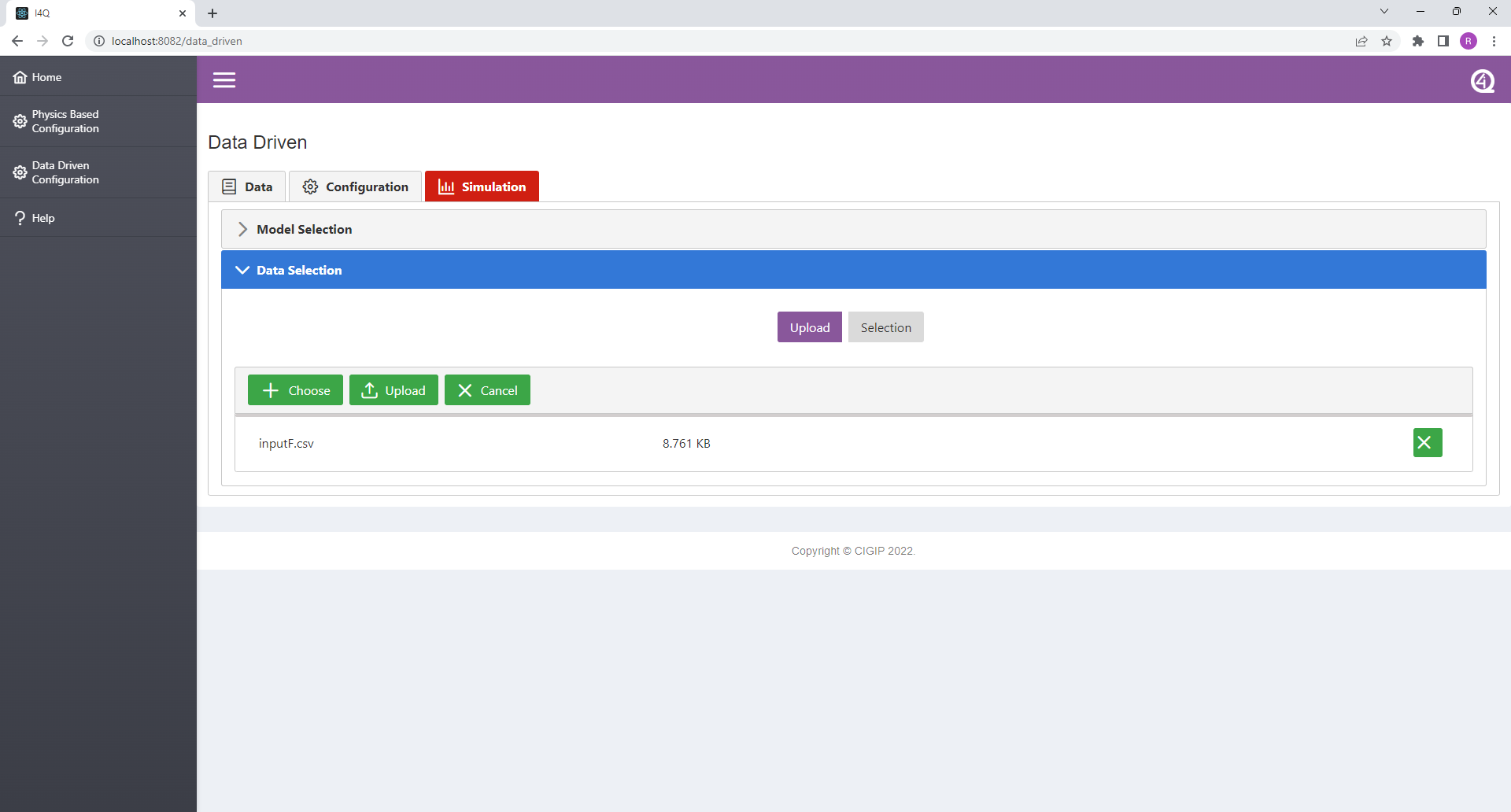
• Uploading Data files (Data TAB).

1. Click “Choose” button or drag and drop CSV files from your computer.

2. The selected CSV and its size will be displayed as a list.

3. To have this CSV available on the CSVs dropdown list click “Upload” button, otherwise click “Cancel” button to clean the file uploader.

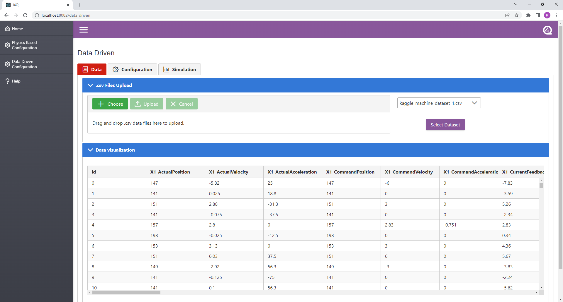
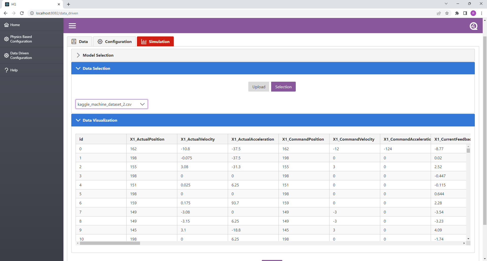
• Selecting a Dataset (Data TAB).

1. Select the desired dataset from the data files dropdown list.

2. Click on “Select Dataset” to select the desired CSV file.

3. Data file can be visualized in table format by opening “Data Visualization” drop-down container. Rows are limited to 200 ocurrencies, full file can not be visualized in solution’s frontend.

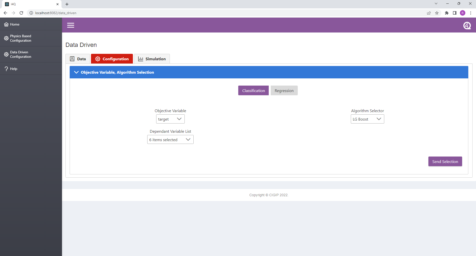
• Selecting Objective Variable and Algorithm (Configuration TAB).

1. Select the type of problem which will be addressed.

2. Select the desired objective variable from the “Objective Variable” dropdown list. If there is a discrepancy between the variable and the type of problem selected, the selected variable has priority.

3. Select the desired dependant variables from the “Dependant Variable List” dropdown list.

4. Select the desired algorihm from the “Algorithm Selector” dropdown list.

5. Click on “Send Selection” to send the data to the backend.

• Algorithm Parameterization (Configuration TAB).

1. Algorithm parameters are displayed in a tree table format. By clicking on “Value” column and depending on the parameters, different input fields will appear to modify these values.

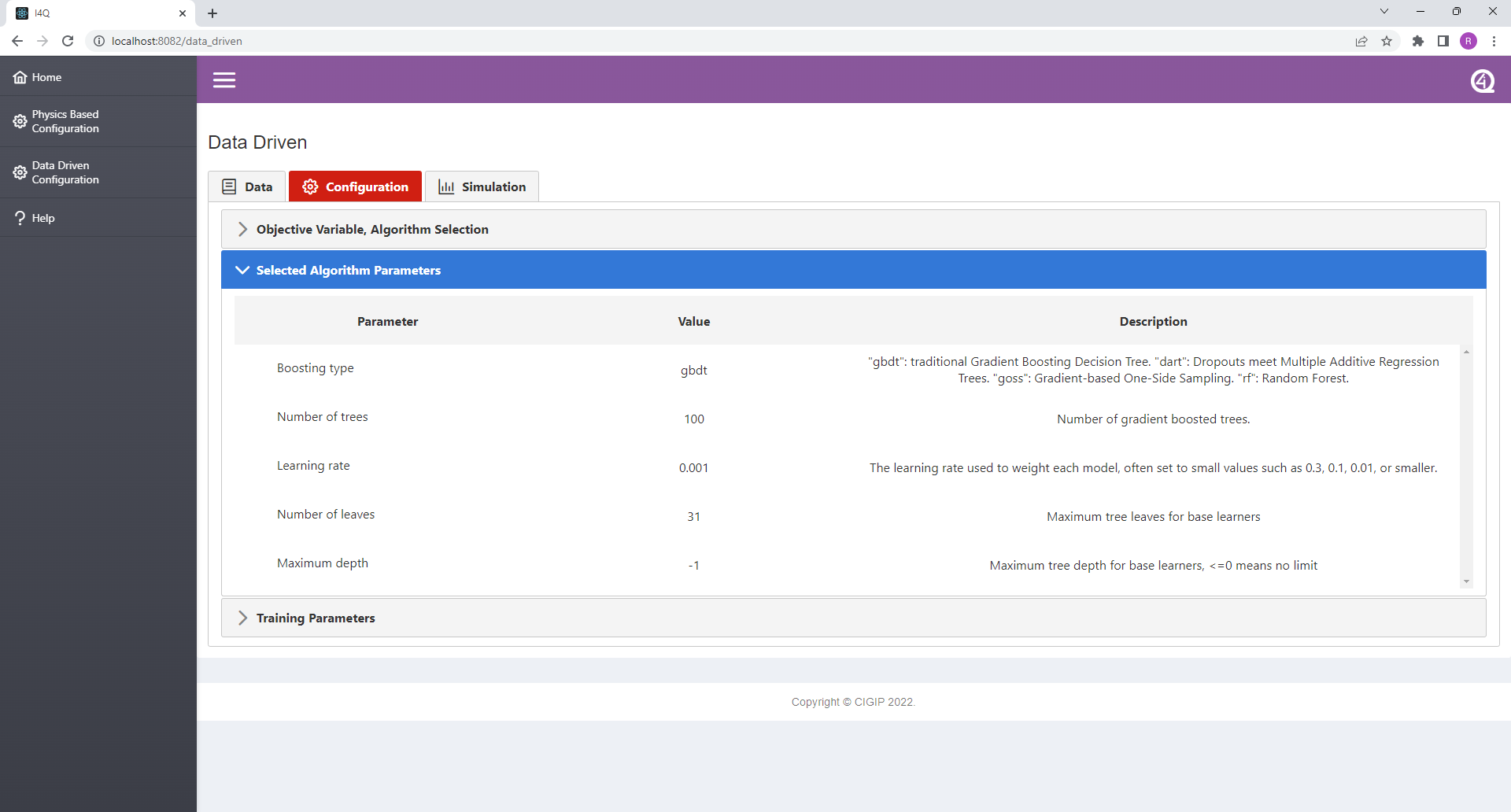
• Training Parameterization (Configuration TAB).

1. Number of splits used for cross-validation can be defined.

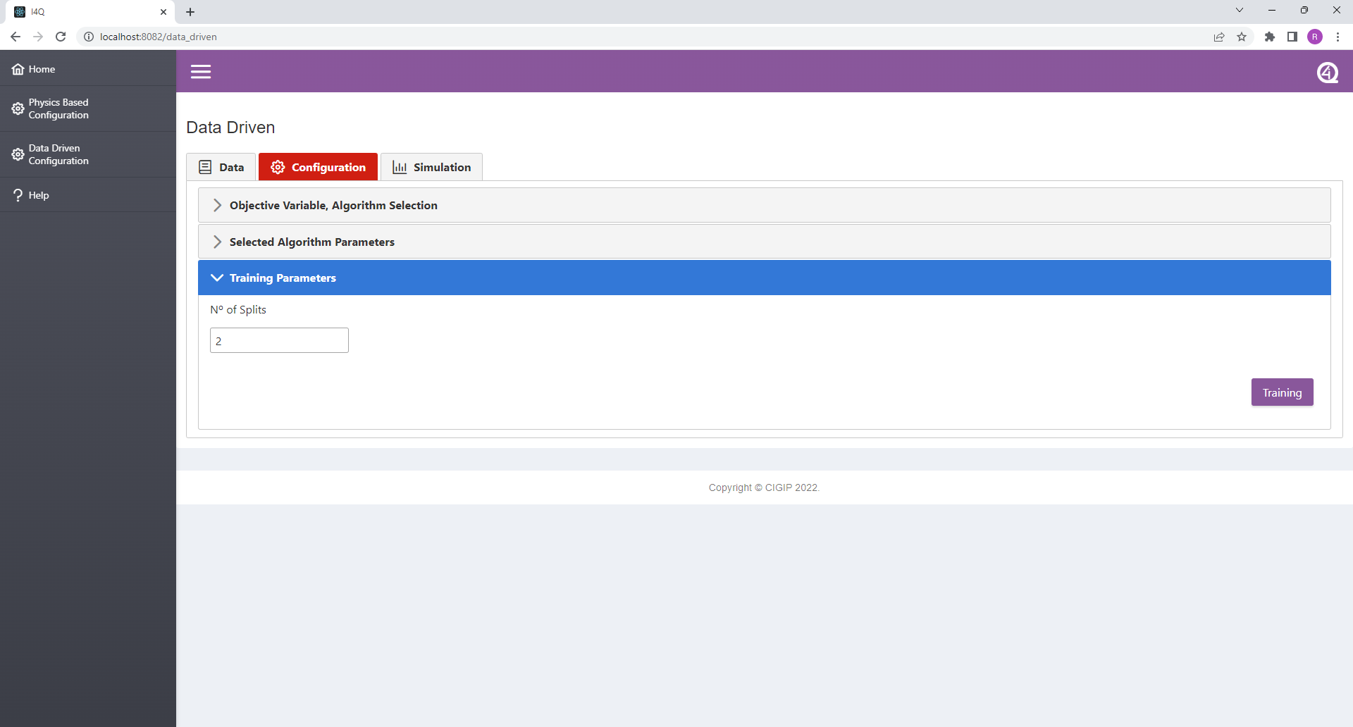
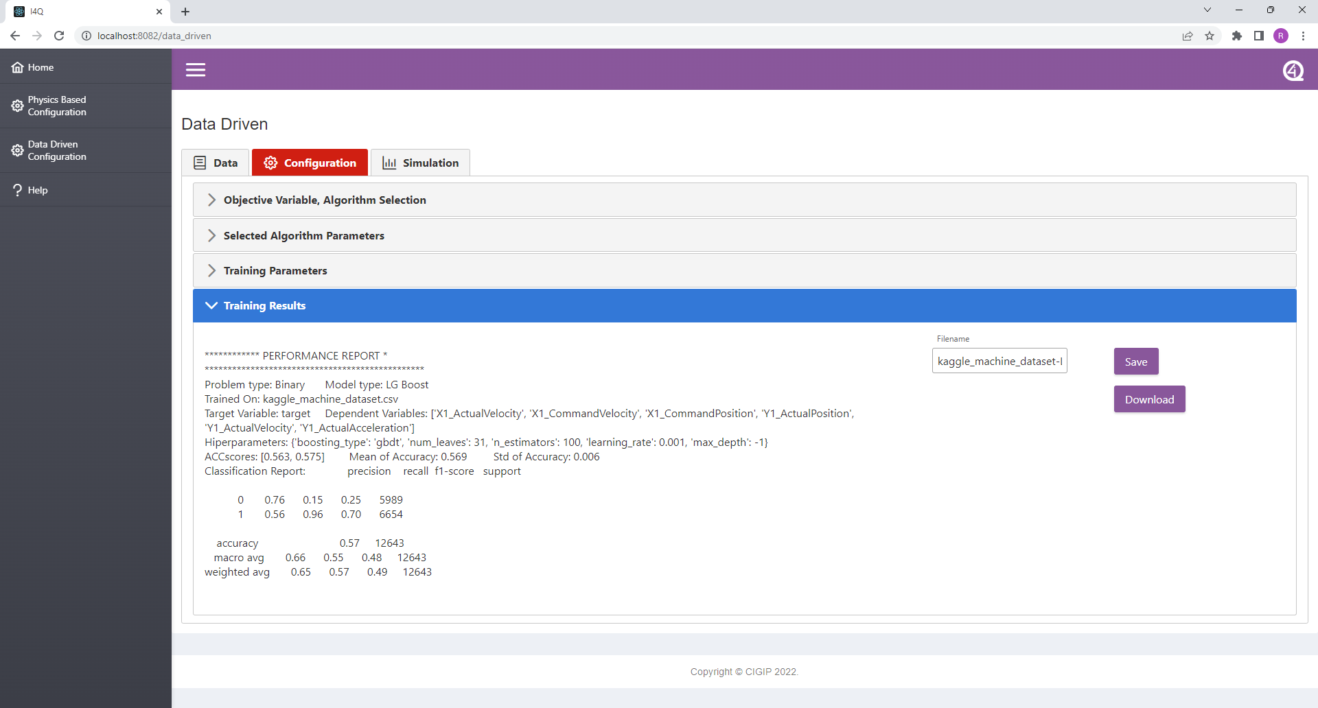
• Training Results (Configuration TAB).

1. Trained model results are shown as a report.

2. These trained model can be saved internally or downloaded as a .pkl file.

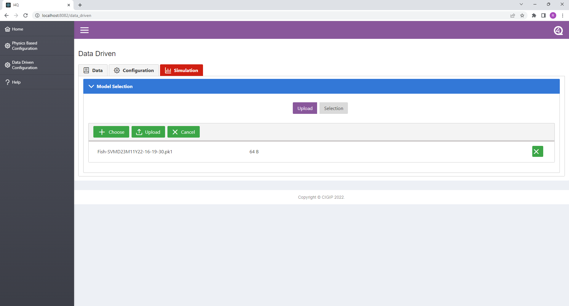
• Uploading Models (Simulation TAB).

1. Click on “Upload” button.

2. Analogously to other file uploaders, users can add models .pkl files.

3. Once selected and uploaded, the model is available in the “Model Selection” dropdown list.

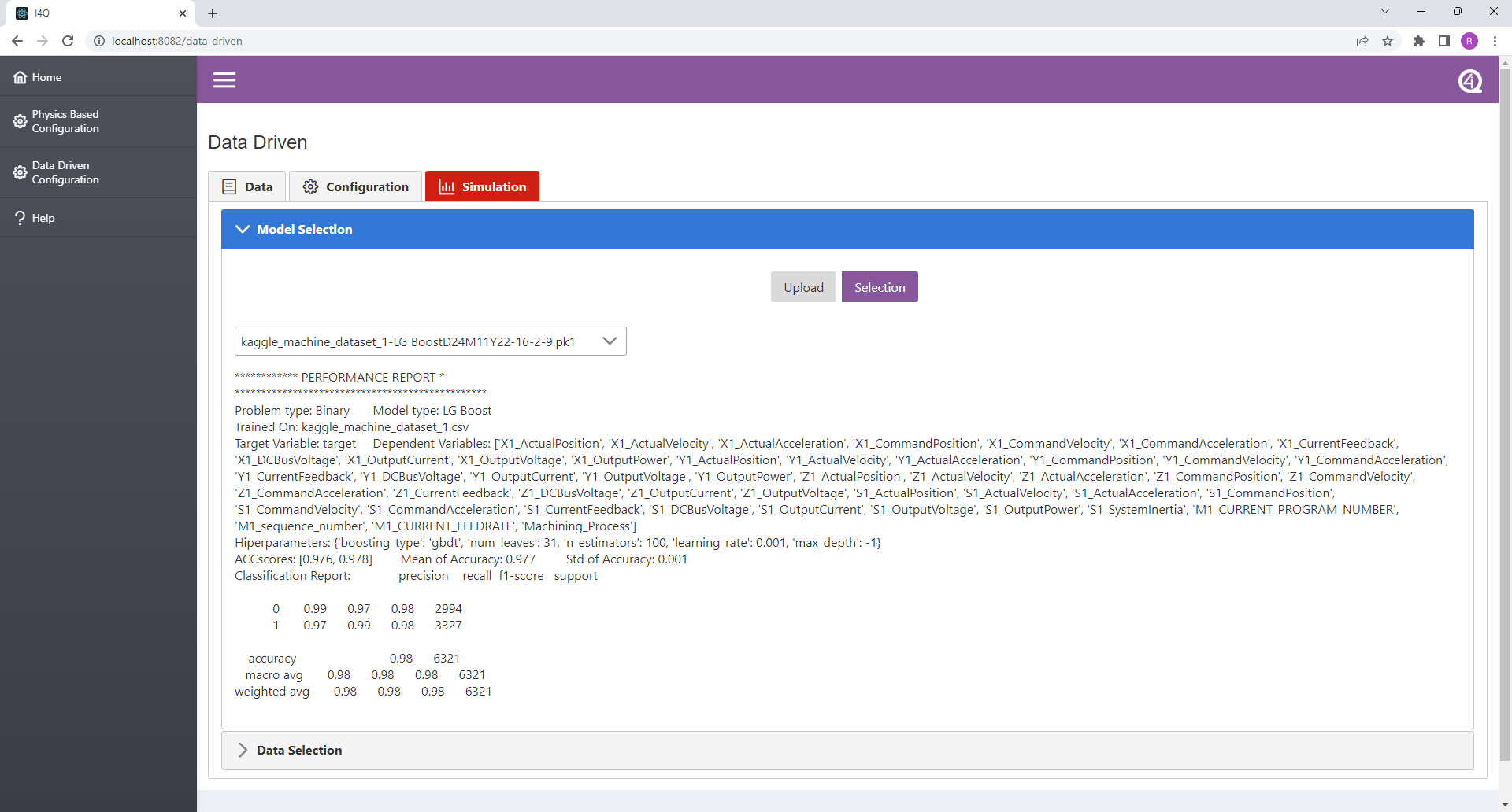
• Model Selection (Simulation TAB).

1. Select the desired model from the “Model Selection” dropdown list.

2. Once selected, the selected model information is displayed.

• Uploading Data Files (Simulation TAB).

1. Click on “Upload” button.

2. Analogously to other file uploaders, users can add .csv data files.

3. Once selected and uploaded, the data file is available in the “Data File Selection” dropdown list.

• Data Selection (Simulation TAB).

1. Select the desired data file from the “Data File Selection” dropdown list.

2. Once selected, data file can be visualized in table format by opening “Data Visualization” drop-down container.

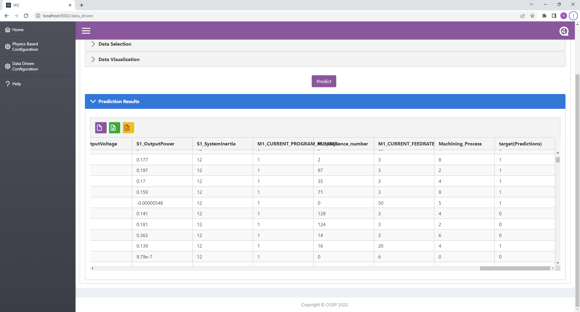
• Prediction Results (Simulation TAB).

1. Click on “Predict” button.

2. Results are displayed in table format. The predictions for the selected objective variable are in the righmost column. Rows are limited to 200 ocurrencies, to see full dataset download it.

3. This data can be downloaded as: .csv, .xlsx and .pdf.

Misc.

If desired, to ease code debugging, install Google Chrome React Developer Tools and Redux DevTools extensions to debug React code and see Redux state. To open developer tools:

CTRL + SHIFT + i

fmiSim Python library User Manual

The fmiSim library is included and managed inside the i4QDT via the proper API functions or the front-end. As such, the following information is only useful for someone who would want to use this library outside i4QDT.

The library contains two main classes: Model and Master. The class Model is used to store the information contained in a FMU file and to give access to its functionality. The class Model is used through two derived classes: ModelCS and ModelME, for fmu CoSimulation FMUs and ModelExchange FMUs respectively. The class Master is an implementation of an orchestrator to carry out CoSimulations. It takes a set of models, a set of connections between their variables and a set of simulation parameters and runs a simulation. More detailed information about CoSimulation, ModelExchange and Function Mock-up Units can be found in https://www.fmi-standard.org/. To create a ModelXX object from file use:

from fmiSim.fmi_models import create_model
filename = "/my_fmu_file.fmu"
model = create_model(method="file", filename=filename)

If the type of FMU is known a priori, the model can be instantiated as:

from fmiSim.fmi_models import ModelCS, ModelME
model = ModelCS.fromfile(filename)
# or
model = ModelME.fromfile(filename)

Once instantiated, a model can be used to retrieve information about the FMU:

parameters = model.parameters
inputs = model.get_variables(filterfunc=lambda x:x.get("causality")=="input",
                              variable_attributes=["name", "valueReference"])
# or
model = ModelME.fromfile(filename)

Every function defined in the FMI standard for a FMU can be used with the Model interface. The class Master is used as the orchestrator for CoSimulation. Therefore it can be used only with CoSimulation FMUs. It can be created from a set of instantiated models and a set of connections between their variables:

from fmiSim.fmi_models import ModelCS
from fmiSim.fmi_master import Master
filenames = ["pulseForce.fmu", "rampForce.fmu","addSignals.fmu","springMassModel.fmu", "gainInput1.fmu"]
# Connections is a list of tuples defining the connection between an output variable of one model and an
# input variable of another
# The name of variable is given by modelIdentifer.variable_name
connections = [("pulseForce.forceOutput", "addSignals.inputSignal1"),
               ("rampForce.rampforceOutput","addSignals.inputSignal2"),
               ("addSignals.signalOutput", "springMassModel.inputForce")]
# Read the models
models = [ModelCS.fromfile(filename) for filename in filenames]
master = Master(models, connections)

To run the cosimulation the method simulate from Master is used. A dictionary specifying simulation options can be supplied to the function:

# Variables to be returned by the simulation
variables_of_interest = ["time", "pulseForce.forceOutput", "rampForce.rampforceOutput",
                         "addSignals.signalOutput", "springMassModel.massForce",
                          "springMassModel.massPosition", "springMassModel.massVelocity"]
options = dict(
    start_time=0.0,
    stop_time=10.0,
    step_size=0.001,
    start_values=dict(
                pulseForce={"pulseForce.startTime":0.2},
                springMassModel={}
                         ),
    results=dict(
            format="structured_array",
            output_variables=variables_of_interest
    ))
results = master.simulate(options=options)

For more detailed information about the usage of the library, check the code examples contained in /examples/examples.py